본 게시물은 University of Arizona의 Prof. J. Scott Tyo의 OPTI512R 강의를 보고 정리한 내용입니다.
전공자가 아닌 만큼 부정확한 정보가 포함되어 있을 수 있습니다.
부정확한 정보가 있다면 알려주시면 감사하겠습니다.
지금 까지 우리는 우리가 다루는 field가 purely monochromatic 하다고 가정하였다. 즉, 그들은 time dependence $e^{j \omega t}$인 ideal complex exponential이었으며, bandwidth가 zero이다. 모든 physical optical field가 radiation을 생성하는 physical process에서 randomness과 관련된 finite bandwidth를 가질 것 이기 때문에 이러한 가정은 현실적이지 않다.
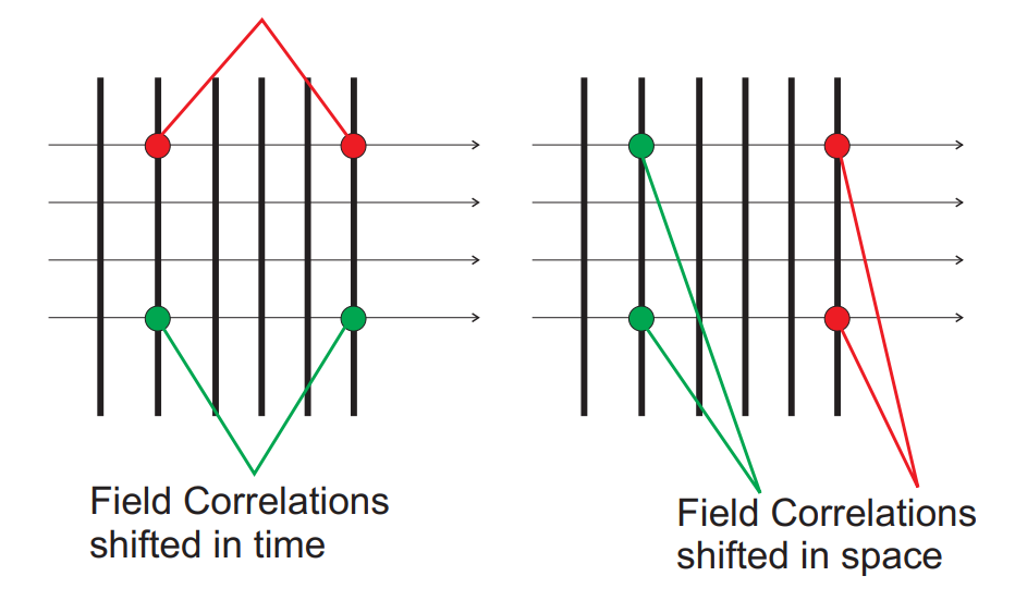
우리가 일반적으로 고려하는 두 가지 종류의 coherence가 있다. 첫 번째 class는 temporal coherence이고, 두 번째 class는 spatial coherence이다. Temporal coherence는 light가 delayed version의 자신을 interfere 하는 ability를 describe 한다. Spatial coherence는 light의 beam이 자신의 shifted version을 interfere하는 ability를 describe한다. 전자를 test하기 위해 두 개의 field copy를 만들고 한 개를 delay 시킨 후, recombine해야한다. 이를 amplitude splitting이라고 한다. 후자를 test하기 위해, 우리는 두 different location의 wavefront를 sampling하고, 그 field들을 comjunction하고, interfere하게 한다. 두 번째 전략은 wavefront splitting interferometry이다. 이러한 개념은 아래 그림에 개략적으로 설명 되어 있다.
Temporal Coherence
우리는 Position $P$와 Time $t$에서의 optical field를 $u(P, t)$로 describe한다. complex field에는 time에 따라 천천히 변하는 complex envelop function $A(P,t)$가 존재한다. 여기서 천천히의 의미가 무엇일까? Field에는 bandwidth $\triangle \upsilon$를 가지고, $A(P,t)$의 time variation은 $1/\triangle \upsilon$정도이다. Time interval $\tau << 1/\triangle \upsilon$에 걸쳐 envelope는 거의 constant 하다. 우리는 coherence time $\tau c \approx 1/\triangle \upsilon$가 filed가 자신과 highly correlated인 time이라고 describe 할 수 있다.
1. Temporal Coherence
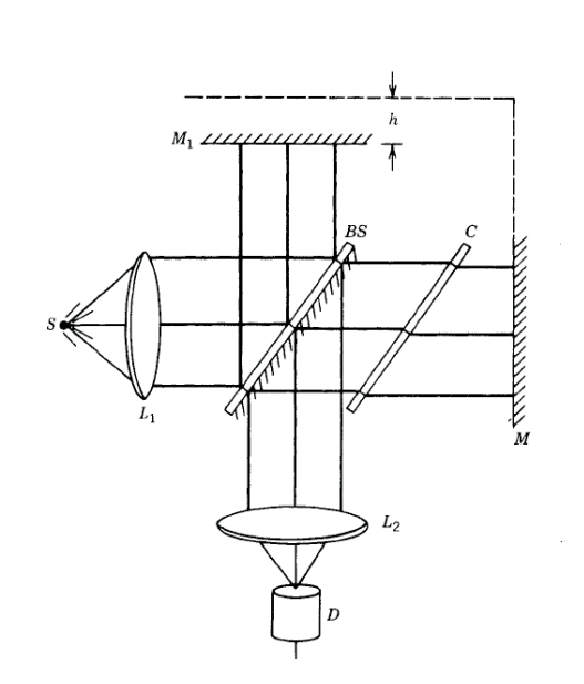
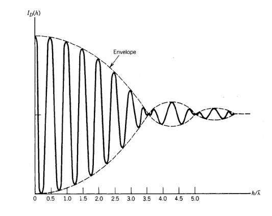
위 그림에 표시된 interferometer를 고려하자. Collimated light는 beam splitter로 들어가 두 개의 path로 split 된다. 두 path 모두, mirror에서 반사되지만 interferometer의 두 arm의 total path length는 path length h 만큼 다르다. compensator는 Beam splitter를 통과하는 두 path사이의 dispersion을 manage 하는 데 사용된다. 두 개의 Mirror에서 reflection 된 후, light는 beam splitter에 두 번째로 부딪힌다. 아래로 향하는 path는 interferometer의 두 arm을 각각 통과한 light의 superposition이다. 두 arm의 path length가 동일하다면, detector에 constructive interference가 발생하고, arm 중 하나에서 path length가 변경되어 두 arm이 다른 path length를 가지게 되면, 이 constructive interference가 감소한다. $h ~ \lambda /2$가 되면, destructive interference 발생하게 된다. 우리가 h를 scan 할 때, light state와 dark state 사이에서 oscillate 하는 fringe를 통과하게 된다. 이러한 oscilating fringe는 아래 그림에서와 같이 source의 bandwidth에 의해 determine 되는 envelope function에 의해 modulate 된다. source에 wavelength가 많으면 각각 아래 그림과 같은 Fringe pattern을 만들고, 이 Fringe pattern들은 서로 superimpose 된다. 모든 Fringe pattern의 summation은 우리가 볼 수 있는 source의 spectral content를 determine 하는 데 사용될 수 있는 interferogram을 생성한다.
Detector에서 record 된 signal은 일부 finite integration time 동안의 averaged total optical field의 intensity에 proportional 하다. 대부분은 아닐지라도 많은 experiment에서, detector의 integration time은 $\tau_c$ 보다 훨씬 크기 때문에, 이 integration process를 infinite time average로 고려할 수 있다. detector의 intensity는 다음과 같다.
$$I_D (h) = \bigg < \bigg | K_1 u(t) + K_2 u(t + {2h \over c})\bigg |^2 \bigg >$$
여기서 $K_1$과 $K_2$는 interferometer의 두 arm에 있는 loss를 설명하는 real constant이고, $u(t)$는 light가 collimated 되기 전에 point source에서 emit 되는 signal이다. Angle bracket은 infinite time average를 의미한다. 우리는 이것을 다음과 같이 expand 할 수 있다.
$$I_{D}(h)=K_{1}^{2}\left\langle|u(t)|^{2}\right\rangle+K_{2}^{2}\left\langle\left|u\left(t-\frac{2 h}{c}\right)\right|^{2}\right\rangle+2 K_{1} K_{2} \operatorname{Re}\left[\left\langle u(t) u^{*}\left(t-\frac{2 h}{c}\right)\right\rangle\right]$$
처음 두 term은 모두 infinite time average 이므로 우리는 다음을 define 할 수 있다.
$$I_o = \big < |u(t)|^2 \big > = \bigg < \bigg | u(t-{2h \over c}) \bigg |^2 \bigg >$$
세 번째 term은 $u(t)$로 describe 된 analytic signal의 autocorrelation function $\gamma_u(\tau)$으로 인식하며, 여기서 $\tau = 2h/c$는 interferometer의 두 arm에서의 time delay이다. 우리는 Autocorrelation function의 Fourier Transform이 field의 (real) power spectral density라는 것을 이미 배웠다. Interferogram의 Measurement는 우리가 source의 spectrum을 Fourier transform을 통해 확인할 수 있게 해 준다. 이 method는 Fourier Transform spectroscopy으로 널리 알려져 있다.
Autocorrelation function의 normalized version을 사용하는 것이 종종 유용하다. 우리는 light의 complex degree of coherence를 다음과 같이 정의할 수 있다.
$$\mu(\tau) = {\gamma_u(\tau) \over \gamma_u(0)}$$
우리는 모든 $\tau$에 대해 $\mu(0) = 1$이고, $\mu \tau \leq 1$이라는 것에 주목해야 한다. 위 그림을 다시 보면, $\tau$가 낮은 경우 coherence가 크고, Fringe modulation이 작은 큰 $\tau$에 대해서는 coherence가 0으로 떨어지는 것을 알 수 있다. $\gamma_u$는 일반적으로 phase가 $90^{\circ} $인 real part와 imaginary part를 갖기 때문에 coherence의 정도는 fringe의 envelope와 관련이 있다는 점에 유의해야 한다. 우리가 Fringe pattern으로 갈수록, path length difference가 커지며, 두 beam의 interfere ability가 $2h/c > \tau c$까지 낮아지고, field 도 더 이상 conherent하지 않게 된다.
2. Spatial Coherence
Temporal coherence에 대해 논의할 때, 우리는 모든 source가 finite bandwidth를 가져야 하므로, field가 더 이상 스스로와 interferes하지 않는 time 이후에 coherence time으로 알려진 time이 있다는 점에 주목하였다. 그 Analysis를 수행하면서, 우리는 radiation의 source가 infinitesimal point source라고 가정했다. 물론, 모든 real source는 finite spatial extent를 가질 것이며, source의 다른 부분에서 emit 되는 light의 pakcet이 반드시 서로 coherent 한 것은 아니다. 이것은 spatial coherence의 concept으로 우리를 이끈다. Time delay 없이 두 point $P_1$과 $P_2$에서 observe 되는 signal $u(P_1, t)$와 $u(P_2, t)$를 고려하자. $P_1 = P_2$일 때, field는 perfectly correlate 하다. 그러나 $P_2$가 $P_1$에서 멀어질수록 correlation이 lost 되고, 이는 light의 spatial coherence가 limit 된다는 것을 의미한다.
Light의 spatial coherence를 탐구하는 classic experiment는 아래 그림에 묘사된 Young's experiment이다. spatial 하게 extend 된 source $S$는 point $P_1$과 $P_2$에 두 개의 small pinhole이 있는 opaque screen을 illuminate 한다. 이 light은 pinhole을 통과해 light가 interfere 할 수 있는 viewing screen으로 모여든다. Pinhole을 통해 viewing screen으로 propagate 될 때, Pinhole을 통과하는 light는 각각 $r_1/c$와 $r2/c$의 delay를 겪는다. Delay time $(r_2 - r_1)/c < \tau_c$일 때, 우리는 interference가 있을 것으로 예상할 수 있고, 우리는 expect fringe를 expect 할 수 있다. 이 fringe의 depth는 두 pinhole을 통과하는 field 간의 correlation에 따라 달라진다.
우리는 observation screen의 point $Q$에 도달하는 light의 intensity를 계산하고자 하고, observation time이 infinite 하다고 가정하여 infinite average를 사용할 것이다. Intesity는 다음과 같이 표현된다.
$$I(Q) = <U^*(Q,t)u(Q,t)>$$
$I(Q)$를 evaluate 하려면, $Q$의 field를 pinhole의 field로 표현해야 한다. 우리의 scalar diffraction theory에서, 우리는 두 pinhole에 있는 field의 weighted superposition으로 field를 다음과 같이 쓸 수 있다.
$$u(Q, t) = K_1u \bigg (P_1, t − {r_1\over c}\bigg)+ K_2u\bigg ( P_2, t − {r_2 \over c}\bigg)$$
위 수식에서 $K_1$과 $K_2$는 complex constant이고, $r_1$과 $r_2$는 두 pinhole로부터 $Q$까지의 거리이다. light가 narrow band이고 pinhole이 너무 크지 않다면, 우리는 다음을 쓸 수 있다.
$$K_1 \approx \int\int {\cos\theta_1 \over j\lambda r_1} dS_1 \\K_2 \approx \int\int {\cos\theta_2 \over j\lambda r_2} dS_2$$
이러한 expression들을 작성하면서 우리는 pinhole이 너무 작아서 field가 그들의 spatial extent에 걸쳐 effectly constant 하다고 가정했다. 이 정보를 사용하여 우리는 $Q$에서의 intensity를 다음과 같이 작성할 수 있다.
$$I(Q)=\left|K_{1}\right|^{2}\left\langle\left|u\left(P_{1}, t-\frac{r_{1}}{c}\right)\right|^{2}\right\rangle+\left|K_{2}\right|^{2}\left\langle\left|u\left(P_{1}, t-\frac{r_{2}}{c}\right)\right|^{2}\right\rangle+2 \operatorname{Re}\left[K_{1} K_{2}^{*} u\left(P_{1}, t-\frac{r_{1}}{c}\right) u^{*}\left(P_{2}, t-\frac{r_{2}}{c}\right)\right]$$
또한 우리는 위 수식의 term을 다음과 같이 모을 수 있다.
$$\begin{aligned}
I^{(1)}(Q) &=\left|K_{1}\right|^{2}\left\langle\left|u\left(P_{1}, t-\frac{r_{1}}{c}\right)\right|^{2}\right\rangle \\
I^{(2)}(Q) &=\left|K_{2}\right|^{2}\left\langle\left|u\left(P_{2}, t-\frac{r_{2}}{c}\right)\right|^{2}\right\rangle \\
\gamma_{12}(\tau) &=\left\langle u\left(P_{1}, t+\tau\right) u^{*}\left(P_{2}, t\right)\right\rangle
\end{aligned}$$
두 개의 term은 $Q$에서 1번 pinhole이나 2번 pinhole만을 열었을 경우 얻을 수 있는 intensity이고, 마지막 term은 1번 Pinhole과 2번 pinhole을 통해 screen에 도달하는 light의 cross-correlation function이다. 이 function은 optics에서 mutual coherence function이라고 불리며, coherence theory의 fundamental quantity이다.
Imaging systems with coherent and incoherent fields
지금까지 우리는 strictly monochormatic field만을 고려하였고, 이 가정은 지나치게 restrictive 하며, physical하지 않다. 모든 real physical source는 finite bandwidth를 가져야 한다. 이제 우리는 monochromatic field assumption을 relax 하고, quasi-monochromatic field를 고려할 것이다. 일반적으로 우리는 다음을 쓸 수 있다.
$$u(x, y, z;t) = a(x, y, z;t) \cos(\omega t + \phi(x, y, z;t)$$
위 수식에서 amplitude $a(x, y, z;t)$와 phase $phi(x, y, z;t)$가 slowly-varying 하는 time의 real function이라고 가정하자. 이러한 slowly-varying function은 underlying optical frequency의 많은 cycle에 대해 거의 constant 해야 한다. 이는 function으로 describe 될 수도 있고, statistical distribution으로도 describe 할 수 있다. 이 discussion은 우리를 partial coherence theory와 statistical optics theory로 안내한다.
우리는 partial coherence의 많은 aspect를 두 개의 important situation으로 simplify 할 것이다.
1. Spatially coherent
$$a(x, y, z;t) = a_1(x, y, z)a_2(t) \\
\phi(x, y, z;t) = \phi_1(x, y, z) + \phi_2(t)$$
위 두 수식은 space의 모든 point가 time에 따라 uniform 하게 varying 한다는 것을 알려준다. phase와 amplitude는 사실 position의 function이지만 임의의 두 point에서의 relative amplitude와 relative phase는 fix 되어 있다. 이 경우 모든 impulse response $\tilde h(x_i, y_i; x_o, y_o)$은 동시에 varying 하며, complex field amplitude를 더해야 한다. 이 경우 problem은 complex field amplitude에서 linear 하다.
2. Spatially incoherent
$$\left\langle a\left(\mathbf{r}_{1} ; t\right) a\left(\mathbf{r}_{2} ; t\right) e^{j\left(\phi\left(\mathbf{r}_{1} ; t\right)-\phi\left(\mathbf{r}_{2} ; t\right)\right)}\right\rangle \propto \delta\left(\mathbf{r}_{1}-\mathbf{r}_{2}\right)$$
Notation $<f(x)>$은 function의 average(statistically)를 의미한다. Average는 space, time, frequency 또는 일부 다른 independent variable에 걸쳐 있을 수 있다. 위 수식은 $\mathbf{r}_{1} = \mathbf{r}_{2}$일 때 만, 0이 아니므로, 두 개의 다른 position에서 amplitude와 phase가 completely statistically independent 하다는 것을 알려준다.
Incoherent case의 경우 모든 Impulse response $\tilde{h}(x_i, y_i;x_o, y_o)$는 statistically independent 하다. 우리가 두 field의 superposition의 intensity를 계산할 때, 우리는 다음을 얻는다.
$$<|u1 + u2>= <|u1|^2> +<|u2|^2>+2Re<u_1 {u_2}^*>$$
앞서 설명한 statistical property로 인해, 위 수식의 마지막 term은 0이다. 이는 intensity가 더해진다는 것을 말해준다. Incoherent case의 경우, problem은 intensity에 대해 linear 하다.
'Optics > 이론' 카테고리의 다른 글
| Lec 23. Performance Comparison between Coherent and Incoherent Imaging Systems (0) | 2021.08.31 |
|---|---|
| Lec 22. Coherent and Incoherent Imaging System/CTF/OTF/MTF/PSF (0) | 2021.08.31 |
| Lec 20. Physical Optics Description of Imaging System (0) | 2021.08.27 |
| Lec 19. Fourier Transforming Properties of Lenses and Gaussian Cavities (1) | 2021.08.26 |
| Lec 18. Fresnel Diffraction from Circular Apertures (0) | 2021.08.26 |