본 게시물은 University of Arizona의 Prof. J. Scott Tyo의 OPTI512R 강의를 보고 정리한 내용입니다.
전공자가 아닌 만큼 부정확한 정보가 포함되어 있을 수 있습니다.
부정확한 정보가 있다면 알려주시면 감사하겠습니다.
Comparison of Coherent and Incoherent Imaging
이전 Lecture에서 우리는 Coherent imaging에 해당하는 low-pass filter가 pupil function에 의해 주어지는 반면, 동일한 system으로 Incohernet imaging을 위한 LPF는 pupil의 Autocorrelation function에 의해 주어진다는 것을 보았다. OTF가 0이 되는 Frequency는 CTF가 0이되는 Frequency의 2배이며, 이는 더 높은 spatial frequency field가 System을 통과할 수 있음을 의미한다. 그러나 Binary pupil의 경우, 일반적으로 CTF의 pass band가 OTF의 pass band보다 flatten 하므로, Pass Frequency가 더 나은 contrast를 유지한다. 이러한 problem 및 더 많은 problem들은 두 type의 imaging의 comparison을 어렵게 한다.
Frequency Spectrum of the Image Intensity
직접 compare 할 수 있는 두 가지 System class의 한 가지 aspect는 Image intensity의 Frequency spectrum이다. Incoherent System은 Intensity가 Linear 하지만, Coherent System의 Intensity는 highly nonlinear 하다. 이로 인해 후자의 경우 Frequency spectrum을 찾는 것이 다소 까다로워진다.
Incoherent case에서 Image intensity는 다음과 같은 Convolution Equation으로 define 된다.
$$I_i = |\tilde h|^2 ∗ I_g = |\tilde h|^2 ∗ |u_g|^2$$
대조적으로, Coherent case의 경우 다음과 같은 Intensity를 가진다.
$$I_i = |\tilde h ∗ u_g|^2$$
만약 우리가 Correlation을 represnet 하기 위해 Symbol $\otimes$을 사용한다면 다음을 얻는다.
$$Incoherent : \mathcal{F} \{I_i\} = [H \otimes H][U_g \otimes U_g] \\ Coherent : \mathcal{F} \{I_i\} = HU_g \otimes HU_g$$
이때 $U_g$는 $u_g$의 Spectrum이고, $H$는 CTF이다.
위 두 수식은 Image frequency content의 aspect에서 어느 imaging class가 더 나은지에 대한 결론을 이끌어 내지 못한다. 그러나 두 사례의 frequency content가 상당히 다를 수 있다는 점을 확실히 보여준다. 또한 둘 사이의 모든 comparison은 Fourier space의 amplitude 및 phase distribution에 따라 달라진다.
Intensity transmittance는 같지만, phase distribution은 다른 두 distribution의 간단한 예를 알아보도록 하자. 이 중 하나는 coherent ligth를 통해 better image를 얻을 수 있고, 다른 하나는 Incoherent ligth를 통해 better image를 얻을 수 있다. 두 경우 모두 Intensity transmittance는 다음과 같다.
$$\tau(x,y) = \cos^2(2\pi \xi_0 x)$$
여기서 우리는 $(\xi_c /2) \leq \xi_0 \leq \xi_c$라고 가정했고, $\xi_c$는 coherent cutoff frequency이다. 두 object는 다음의 amplitude transmittance를 가진다.
$$t_a(x_1,y_1) = \cos2\pi \xi_0 x_1 \\ t_b(x_1, y_1) = |\cos 2\pi \xi_0 x_1|$$
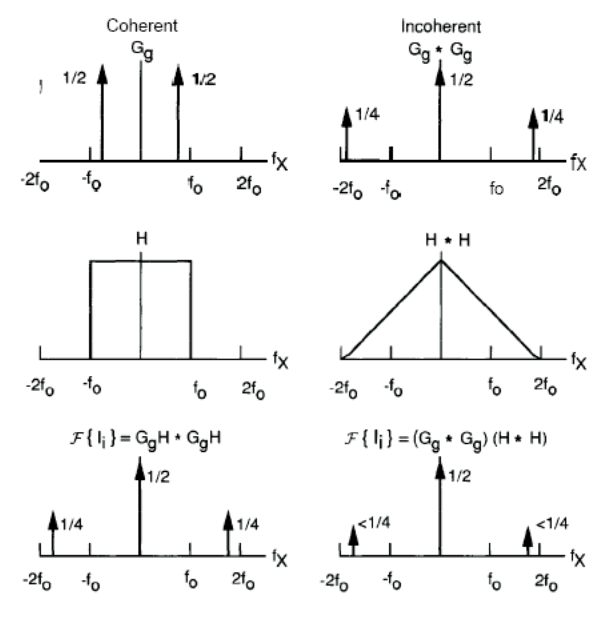
아래 그림은 obejct A에 대해 $\otimes$를 사용해 정의한 operation을 수행하는데 필요한 operation을 보여준다. 우리는 System이 모든 case에서 diffraction limit를 가진다고 가정해 왔다. Final result에서 Final image의 contrast가 incoherent illumination인 경우 더 나쁘다는 것을 알 수 있으므로, 이 경우 Coherent illumination이 더 낫다고 할 수 있다.
Object B의 경우 object는 frequency $2\xi_0$으로 periodic 하며, 이는 amplitude의 fundamental frequency 또한 $2 \xi_0$임을 의미한다. 그러나 $2\xi_0 > \xi_c$인 경우 Coherent system의 cutoff frequency이므로, Coherent illumination의 경우 contrast가 전혀 없다. 분명히 Incoherent illumination은 Case B에 더 좋다.
Two-Point Resolution
System이 resolve 하기를 원하는 두 개의 closely-spaced point source를 고려하자. Aperture는 diameter가 L인 circular pupil이라고 가정한다. 두 point source가 poisiton$(x, y) = (\pm \delta/2, 0)$에 있다고 가정하고, Image plane의 x-axis를 따라 image를 고려할 것이다. Diffraction-limited imaging에 대한 Rayleigh-criterion은 한 source에서 Airy disk의 first null이 다른 source의 image location에 정확히 떨어질 때 두 point source를 거의 analysis 할 수 없다고 주장한다. 이 Distance는 다음과 같다
$$\delta = 1.22 {\lambda d_i \over L}$$
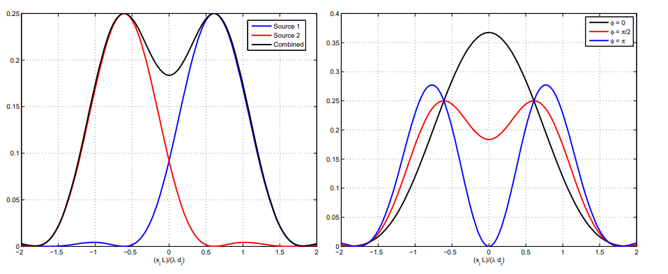
이 경우 x-axis를 따라 coherent intensity distribution은 다음과 같다.
$$I_c(x) \propto somb (x − 0.61) + e^{j\phi}somb (x + 0.61)|$$
이때, $\phi$는 두 가지 coherent source 사이의 relative phase difference이다. 반대로, source가 Incoherent 하면 우리는 다음과 같은 intensity distribution을 가진다.
$$I_i(x) \propto somb (x − 0.61)^2 + somb (x + 0.61)^2$$
아래 그림은 이 두 distribution에서 세 가지 다른 $\phi$값에 따른 결과를 plot 한 것이다,
Two-Point Resolution
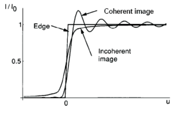
Coherent system과 Incoherent System을 compare 하는 몇 가지 다른 effect가 존재한다. 그러한 effect 중 하나는 step-response이다. system이 rectangular exit pupil을 가지고 있다고 가정하자. Knife-edge(step function)에 대한 이 system의 response는 위 그림에 나와있는 것과 같다. Two-dimensional intensity에 해당하는 image는 아래 그림에 나타나 있다.
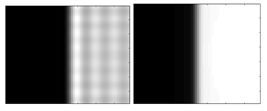
이 두 가지 response를 보면, coherent image가 더 sharper 하다고 말할 수 있으며, 이는 intensity transition이 더 sharp 해졌다는 것을 의미한다. 그러나 discontinuity와 associate 된 ringing도 있다. Incoherent image의 경우 Blurrier 하게 보이지만, ringing이 없다. 또한 두 경우에서 50% point의 apparent location은 다소 다르다.
Speckle
Coherent illumination을 사용할 때, 고려해야 할 또 다른 important consideration이 존재하는데, 그것은 바로 Speckle effect이다. 우리가 Analysis를 수행할 때, Object transmission function, Lens transmission function 및 Propagation distance가 정확하게 알려져 있다고 가정했다. 그러나 Real system에서 이러한 object는 모두 Thickness, smoothness, orientation, index of refraction등에서 random variation을 가지며, order of wavelength(혹은 더 많은 case)에 따라 vary 하기도 한다. 이 Randomness의 effect는 다음과 같은 question에서 object의 transfer function에 random phase variation을 도입하는 것이다.
$$\tau (x_1, y_1) = t(x_1, y_1)e^{j\phi}(x_1,y_1)$$
여기서 $\phi(x_1, y_1)$은 question의 process를 describe 하는 random number이다.
Coherent illumination을 사용하면, aperture의 각 point에 의해 diffraction 된 field amplitude가 phase에 추가된다. 어떤 region에서 constructively add up 하고, 다른 region에서는 destructively add 한다. 이 additional random phase의 effect는 object에 대한 각 point의 contribution을 dephase 하는 것이다. 이 raondomness statistic에 따라 real image 앞에 "Speckle" noise를 넣는 강력한 position function을 도입할 수 있다.
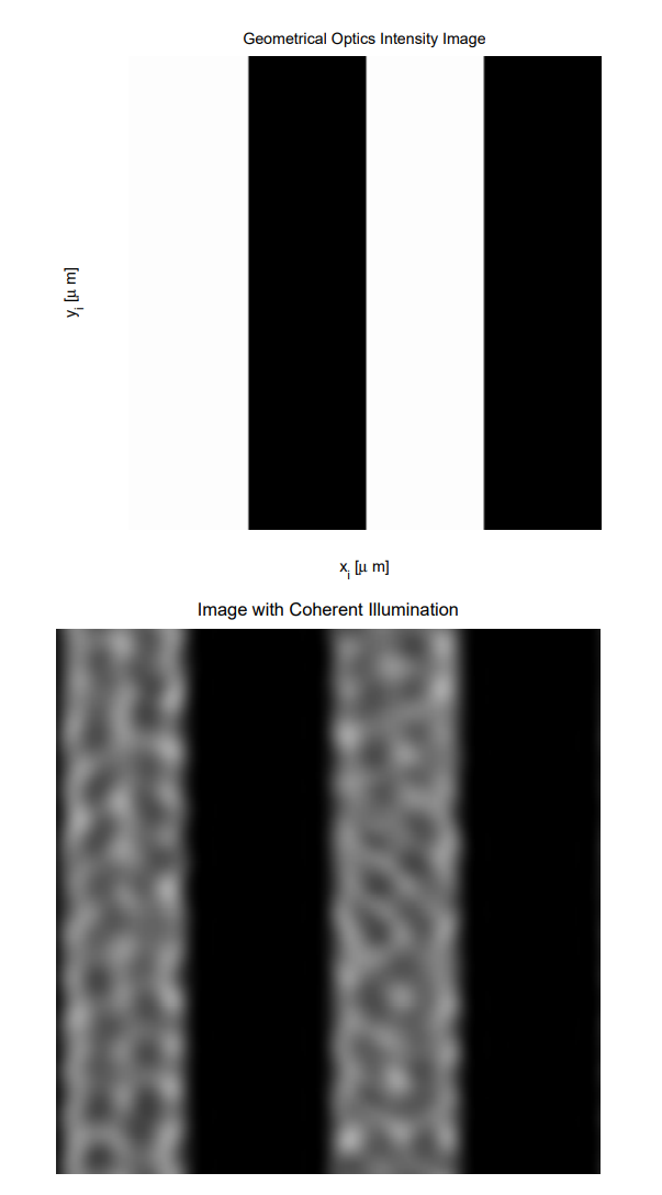
아래 그림에 표시된 object를 고려해보자. Ideal grating을 다음과 같이 describe 할 것이다.
$$t(x, y)=1+ \alpha sgn [sin(2\pi\xi_0x)]$$
Phase $\phi(x_1, y_1)$을 $\pi/4$ surface torlerance에 해당하는 $\pi/4$의 standard variation을 가지는 Gaussian random variable이 되도록 할 것이다. 이 small amount의 phase uncertainty는 아래 그림과 같이 grating image 위에 speckle pattern으로 나타난다.
'Optics > 이론' 카테고리의 다른 글
| Lec 24. Effect of Aberration on the Performance of Imaging System (0) | 2021.08.31 |
|---|---|
| Lec 22. Coherent and Incoherent Imaging System/CTF/OTF/MTF/PSF (0) | 2021.08.31 |
| Lec 21. Coherence of Optical Fields (0) | 2021.08.30 |
| Lec 20. Physical Optics Description of Imaging System (0) | 2021.08.27 |
| Lec 19. Fourier Transforming Properties of Lenses and Gaussian Cavities (1) | 2021.08.26 |